This tutorial has been exported from the ELKI wiki. You may be able to find revised and additional Tutorials there.
This tutorial uses Release 0.4 of ELKI. Other releases will work similar.
We analyze the "mouse" data set you can find on the DataSets page.
You should have the files "elki.jar" and "mouse.csv".
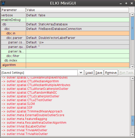
The simplest way is to just run the jar file, either by double-clicking it or by typing "java -jar elki.jar". This will bring an automatically generated graphical UI similar to this:
The window contains three main components. In the top, a tabular view of parameters is presented. Second, a dropdown and a few buttons allow the management of saved settings, in the bottom, a log view will give textual output.
The parameter table will dynamically change as you set parameters, since for example adding an algorithm adds new parameters only applicable to this particular algorithm. The colors encode important information on the paranmeters: green parameters are optional, grey parameters have a default value, while orange parameters are missing before the algorithm can be run.
Starting the GUI will generally result in two errors due to missing parameters: you have to choose at least an input file (the parameter dbc.in) and an algorithm (parameter algorithm).
Often the table edit has input assistance such as a file chooser or a dropdown to select amongst known values for this parameter.
In order to save a setting for later use, type a new name into the dropdown on the left and click on "Save". To load a setting, choose it from the drop down and click on "Load".
Settings are saved in the file MiniGUI-saved-settings.txt that you should find easily editable with any text editor. Individual entries are separated with an empty line, and the first line of each section is the title of the setting, while the remaining lines give the options. The syntax is that of the ELKI command line interface, for easy batch operation.
The log window will provide you with progress information (when you set verbose to true) and other status messages. When the "Run Task" button is grey, you probably have not yet set all required parameters. The log window will report any parameterization errors along with some suggestions on how to set the parameters. In the screenshot above, it gives a list of known algorithms to help you set the algorithm parameter.
We will analyze the mouse data set with two well-known algorithms, k-means-clustering and EM clustering. This data set is a simple to understand example to see a key difference between these two algorithms.
First of all, we set the dbc.in parameter to the input file, mouse.csv. If you click on the table, a button with three dots ... should appear that opens a file selector. Use this to locate the mouse.csv file you downloaded from the DataSets page.
For setting the algorithm parameter, a similar button marked with a plus + is available, that opens a dropdown with algorithms the UI detected:
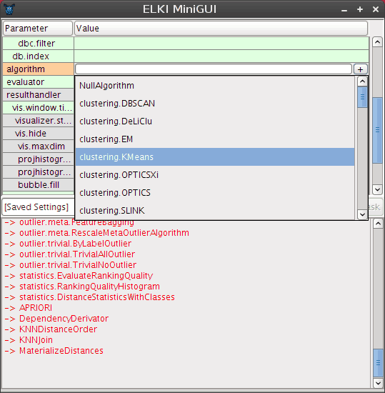
By setting algorithm to clustering.KMeans we choose to use the k-Means clustering algorithm. It will require setting an additional parameter, kmeans.k that will appear below. Set this parameter to 3 for this data set. Leave the other k-Means parameters as is for now: the kmeans.maxiter parameter allows to limit the k-Means runtime, while the kmeans.seed parameter can be used to enforce reproducible results for this algorithm, by using a fixed random generator. We need neither of that for now.
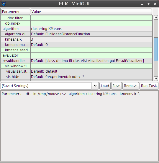
Additionally, we set the parameter evaluator to paircounting.EvaluatePairCountingFMeasure, which will run a standard evaluation method for clustering results. Note that not all evaluators are applicable for evaluating clustering results.
The log window now only gives the command line summary of our parameters, and the Run Task button is now enabled, which we now click to run the algorithm.
After running the algorithm, the GUI by default opens a simple visualization window. This is automatically generated, so the layout is not (yet) the most intuitive, but it does a fairly good job at making visualizations accessible.
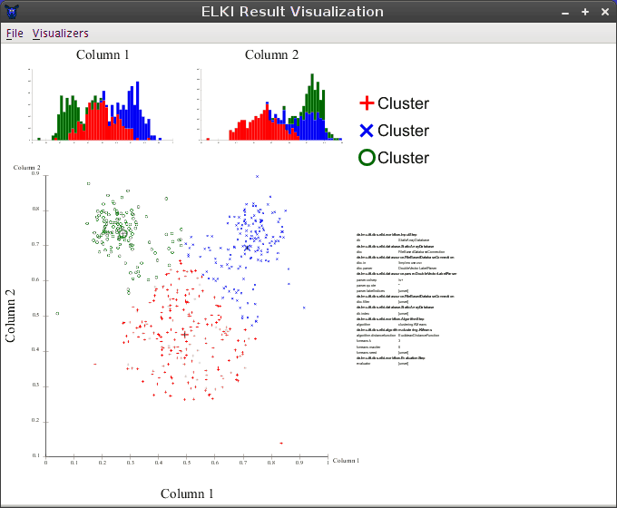
In the main area, three types of visualizations are separated:
The exact arrangement of visualizations depends on a dynamic layouting algorithm and may change with your screen size and your data sets.
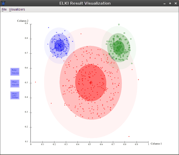
The 2d projection is most interesting for us, and by clicking it we can show it in the full window:
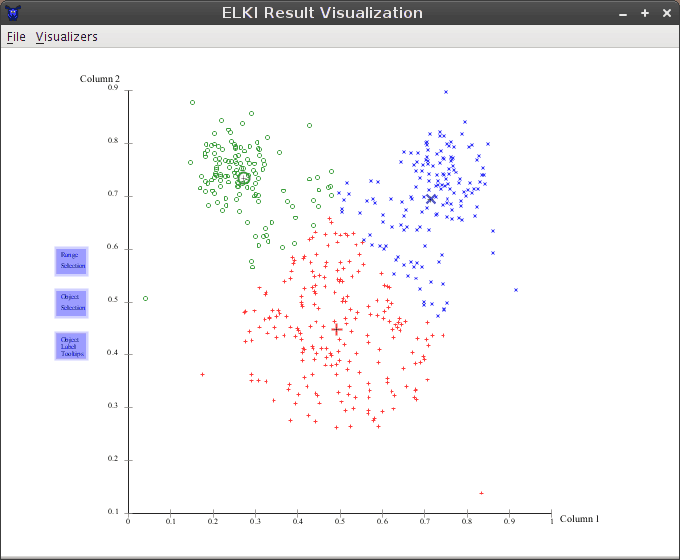
This shows the clustering as obtained by a typical k-Means run. Note that there are three larger symbols, one for each cluster. The larger symbols give the cluster means. In this algorithm, each object is assigned to the cluster where the distance to the mean is the smallest.
To get a more visual impression of the cluster shapes, we can go to the menu and enable the "Cluster Convex Hull Visualization" module for this clustering result:
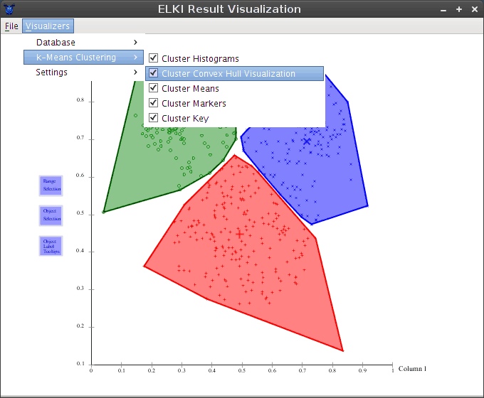
Now you can see more clearly the non-overlapping partitioning produced by this algorithm (more precisely, it produces Voronoi cells. It has a tendency to produce clusters of the same size, which is not appropriate for this data set.
Much more appropriate for this data set is the EM algorithm. Close the visualization window, and replace the value of the algorithm parameter with clustering.EM. For now make sure to replace the value, we don't want to run both k-Means and EM since the overlapping results will be less useful. Again, set em.k to 3, too.
The F-Measure obtained by EM-Clustering is much better, usually around 0.97. This is because this data set consists mostly of three Gaussian clusters, the prime example for EM clustering.
Note that an additional visualizer as automatically enabled to visualize the Gaussian clusters discovered by EM: